We provide two different ways to perform benchmarks: coding or using configuration (CFG) files.
Check the test_fm_benchmark.cpp example.
fm_benchmark.cpp and follow the comments within the code for more instructions.This application allows to configure and run benchmarks very easily. It is implemented in fm_benchmark.cpp and uses the BenchmarkCFG class to parse the CFG files and configure a Benchmark class.
To run a benchmark once compiled:
$ ./fm_benchmark ../data/benchmark.cfg
It will parse benchmark.cfg and run all the solvers in the environment set with the specified configurations. It will generate a folder called results storing a log and grids (if set to do so). This folder will be generated from the current terminal working directory.
benchmark_from_grid.cfg provides an example of most of the capabilites implemented:
# Example configuration file
[grid]
# File: route to image from the current terminal working dir, NOT from this file folder.
file=../data/img.png
#text=../data/map.grid
#ndims=2
#cell=FMCell
#dimsize=300,300
Under grid label, we configure the enviroment. If a file is provided (in occupancy format, that is, 8bits grayscale) FMCell and 2 dimensions will be assumed. dimsize will be adapted to the size of the image given. A 2D FMCell, 200x200 grid is given by default.
file or text, require relative paths using as current folder the current working directory of the terminal executing the benchmark, not the CFG file folder neither the benchmarking program binary folder. [problem] start=150,150 goal=50,50
Start and goal coordinates. Note the format: s_x, s_y, s_z, ... and g_x, g_y, g_z, .... If the goal is omitted, the solvers will be rund through all the possible space.
[benchmark]
name=test_img
runs=5
#savegrid=1
#savegrid=2
Set the name of the benchmark and the number of runs for each solver. If savegrid == 1 a .grid file will be saved for the last run of each solver, identified with solver given name, i.e. FMM.grid. If savegrid == 2 a .grid file is saved for every run identified as <runID>.grid. In both cases, grid files will be stored in a folder results/<benchmark_name>. By default only the log will be saved.
[solvers]
fmm=
fmmstar=
fmmstar=FMM*Dist,DISTANCE
fmmfib=
fmmfibstar=
fmmfibstar=FMMFib*Dist,DISTANCE
sfmm=
sfmmstar=
sfmmstar=SFMM*Dist,DISTANCE
gmm=
gmm=myGMM
gmm=myGMM2,1.5
fim=
fim=myFIM
fim=myFIM2,0.01
ufmm=
ufmm=myUFMM
ufmm=myUFMM2,1001
ufmm=myUFMM3,1001,2.01
Specify the solvers to run. The left-hand size must remain unmodified to correctly identify the solver to use. In the right-hand size constructor parameters could be specified for the different solvers, comma-separated. Note the ordering of the parameters. If other parameters are given, the previous parameteres should be also specified.
The benchmark generates a results/<benmchark_name>.log file which stores the important information. The format is as follows:
First row: benchmark info.
name \t #runs \t #dimensions \t size dim(0) \t size dim(1) \t ... \t #start points \t start index 0 \t start index 1 \t ... \t goal index \
Following rows: solvers information.
runID \t solver name \t time (ms) \n
For instance, the first rows generated by the previous CFG are:
test_img    5       2       400     300     1       60150   20050
0001        FMM     23
0002        FMM     20
0003        FMM     21
0004        FMM     21
0005        FMM     22
0006        FMM*    2
0007        FMM*    0
0008        FMM*    0
0009        FMM*    0
0010        FMM*    0
0011        FMM*Dist        2
...
...
0055        FIM     13
0056        UFMM    15
0057        UFMM    12
0058        UFMM    16
0059        UFMM    12
0060        UFMM    13
Different scripts are provided to help the user to parse the benchmark results. All of them are in the scripts folder and most of them are for Matlab (they have not been tested in Octave but most will probably work).
bm = parseBenchmarkLog(file), where file is the path and filename to the generated log. It returns a cell structure bm with all the information.bm =
name: 'test_img'
nruns: 5
ndims: 2
dimsize: [2x1 double]
startpoints: 60150
goalpoint: 20050
nexp: 60
exp: {12x2 cell}
bm.exp divides the different solvers. For instance, for the previous log, bm.exp{1,1} returns the name of the first solver (FMM) and bm.exp{1,2} the times for all runs for first solver ([23 20 21 21 22]).
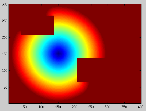
.grid file. Use as `grid = parseGrid('0001.grid')`, gives the result:celltype: 'FMCell - Fast Marching cell' leafsize: 1 ndims: 2 dimsize: [400 300] cells: [300x400 double]
Then, you can easily visualize:
imagesc(grid.cells);
axis image; axis xy;

Every CFG file can run several solvers, with several configurations, several times. However, it only allows to run on one enviroment. To easily solve this, we provide a bash script which executes the benchmark for all the cfg files in a folder (although it could be improved as it assumes the location of the benchmark tool relatively to the terminal working dir).
fast_methods/data/test_cfg/fast_methods/data/Execute run_benchmarks.bash:$ bash ../scripts/run_benchmarks.bash test_cfg
This will generate the folder fast_methods/data/results with the logs of all the benchmarks. In our case, we executed the following CFG files, modifying only the grid size and start point:
[grid]
ndims=2
cell=FMCell
dimsize=150,150    | dimsize=300,300    | dimsize=500,500

[problem]
start=75,75        | start=150,150      | start=250,250

[benchmark]
runs=5

[solvers]
fmm=
fmmfib=
sfmm=
gmm=
fim=
ufmm=
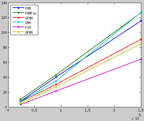
analyzeBenchmark.m from the benchmark folder. Otherwise, you might need to change the path_to_benchmarks variable in the script. The output could be something like:
If you have implemented a custom solver derived from Solver class, you can easily add it to the benchmarking framework. Just follow this steps ("__mysolver__" is meant to be changed by your solver name):
benchmarkcfg.hpp (within readOptions() member function): configure(), set the creation of the solver without parameters: After these changes, you are ready to incude your solver in a CFG file and run the benchmarks.